How to Do a Vlookup in Excel & Google Sheets

Have you ever been overwhelmed by the endless rows of data in Excel? It’s even worse when you’re looking for specific information, and it feels like an endless task to scroll down the rows to find what you actually need. But then, have you pinpointed the right data?

That’s where VLOOKUP in Excel comes to the rescue. With its help, you’ll no longer have to guess. It will find and retrieve the required data for you after completing simple steps.

In this tutorial, I’ll show you how to use VLOOKUP in Excel in different situations to help you avoid the blurry mess you see on your screen.

What is VLOOKUP in Excel? 

In Excel, VLOOKUP is a function used to search for a value in a table and return a corresponding value from another column. The term “VLOOKUP” stands for “Vertical Lookup.” It is commonly used for tasks like retrieving information from a database or creating dynamic reports.

This formula is made of four parameters (or arguments): 

=VLOOKUP(lookup_value, table_array, col_index_num, [range_lookup])

1. lookup_value:

This is the value you want to search for in the first column of your data range. It’s like telling Excel, “Find me this particular piece of information.” For example, if you’re searching for a specific product name or ID, that would be your lookup_value.

2. table_array:

The table_array is the range of cells containing the data you want to search through. It includes the column with your lookup_value and the columns where you expect to find the related information. It’s like defining the playground where Excel should look for the data.

3. col_index_num:

This parameter specifies the column number in your table_array from which to retrieve the data. Once Excel finds the lookup_value, it needs to know from which column to grab the corresponding information. This number starts from 1 for the first column in your table_array.

4. [range_lookup]:

This parameter is optional. If set to TRUE or omitted, VLOOKUP will look for an approximate match. If set to FALSE, it will search for an exact match. Think of it as deciding whether you want an exact match or if you’re okay with something close but not quite identical.

Here is an example for you:

Let’s say you have a table with product names in column A, and prices in column B, and you want to find the price of a specific product named “Widget.” Your formula might look like this:

=VLOOKUP(“Widget”, A2:B100, 2, FALSE)

In this example:

• – lookup_value: “Widget”
• – table_array: A2:B100
• – col_index_num: 2 (because the price is in the second column of the table)
• – range_lookup: FALSE (exact match)

How to use VLOOKUP in Excel 

Using VLOOKUP in Excel involves several steps. Let’s walk through the process. For this tutorial, let’s use the VLOOKUP function to find Sandra Kwon’s employee ID based on her last name.

Step 1: Prepare Your Data

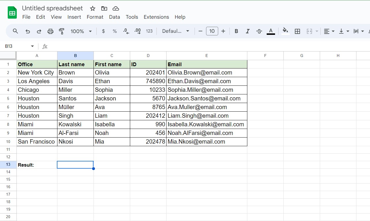
Start with an Excel spreadsheet containing employee names, IDs, and other relevant information. Ensure that your lookup value (last names, in this case) is in the first column of your table array.

Step 2: Locate the Lookup Value

In this example, Ava Muller’s last name is in cell B6. The table array (B2:D10) contains the last names, corresponding employee IDs, and other details.

Step 3: Setting Up the VLOOKUP Formula

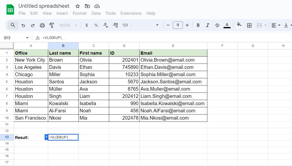
Click the cell where you want Excel to return the employee ID. Let’s say it’s cell B13.

Type =VLOOKUP in cell B13.

Press Enter. Excel will add a left parenthesis after the function, like this: =VLOOKUP(.

Step 4: Inputting Parameters

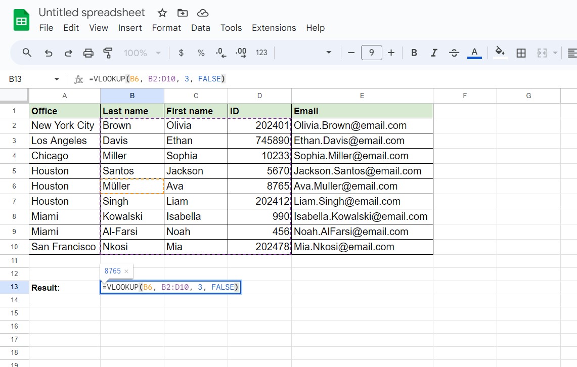
Immediately after the parenthesis, input the following parameters, separating each with a comma:

• – Lookup value: B6 (Sandra Kwon’s last name).
• – Table array: B2:D10 (where your data is located).
• – Column index number: 3 (as the employee IDs are in the third column of the table array).
• – Range lookup: Enter FALSE for an exact match.

Your formula should now look like this: =VLOOKUP(B6, B2:D10, 3, FALSE).

Step 5: Getting the Result

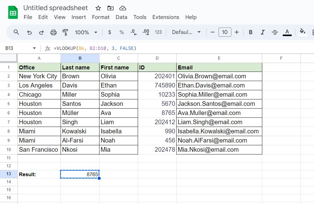
Press Enter. Excel will immediately return the corresponding employee ID for Sandra Kwon, for example, 8765.

Updating Email Addresses with VLOOKUP in Excel

Let’s say Sheet 1 of our demo workbook is our primary spreadsheet, containing comprehensive employee data. Sheet 2, on the other hand, is a secondary spreadsheet with only employee names and their updated company email addresses.

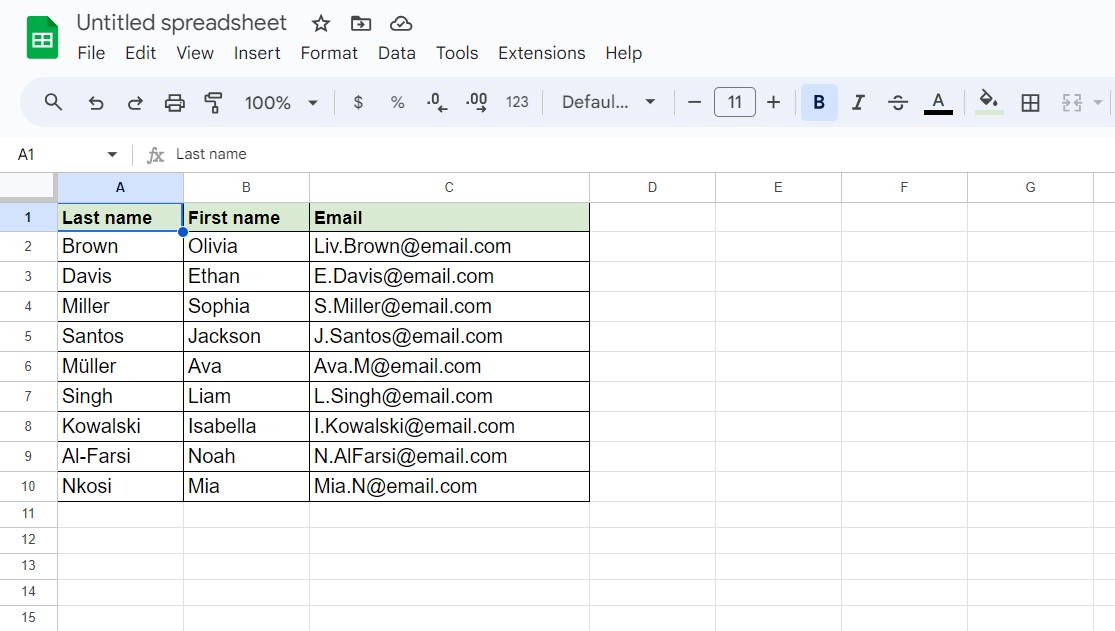
Step 1: Identify the Data and Purpose

You need to update the email addresses in Sheet 1 with the new email addresses from Sheet 2.

Step 2: Understand the Modified VLOOKUP Formula

To return a value from another sheet within the same workbook, use the modified VLOOKUP formula:

=VLOOKUP(lookup_value, sheet!range, column_index_number, range_lookup)

Step 3: Use VLOOKUP to Update Email Addresses

Let’s update the email address in cell E2 of Sheet 1 with the email address in cell C2 of Sheet 2.

Click cell E2 of Sheet 1.

Enter the following formula:

=VLOOKUP(B2, Sheet2!$A$2:$C$10, 3, FALSE)

• – B2: Lookup value (employee name) in Sheet 1.
• – Sheet2!$A$2:$C$10: Cell range in Sheet 2 containing employee names and updated email addresses.
• – 3: Column index number (the email addresses are in the third column of the range).
• – FALSE: Range lookup set to FALSE for an exact match.

Press Enter or Return.

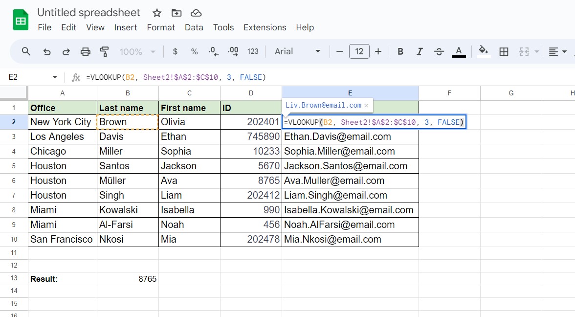
Step 4: Verify the Result

Excel returns the corresponding value from Sheet 2 in cell E2 of Sheet 1: [email protected].

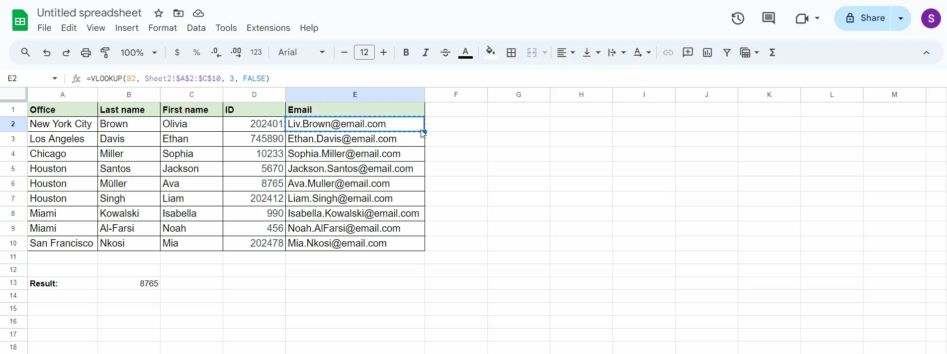
Step 5: Update Remaining Email Addresses

To quickly update the remaining email addresses in Sheet 1, drag the fill handle from cell E2 down. This copies the formula to other cells, updating the email addresses based on the employee names.

---

Automate & scale time-consuming tasks like never before